
It’s been quite a ride in 2026 – economically, militarily, and politically. Hang on – the ride has just begun. This report focuses on the economic ups and downs thus far in 2026 with economics, U.S. military operations, and politics all intertwined. U.S. military operations and politics have significant impacts on the economy. As a result, this report will discuss the performance of a wide variety of economic variables, including: 1) tariffs and trade, 2) the labor market, 3) oil prices, 4) inflation, 5) economic growth, 6) the financial markets, and 7) U.S. debt and deficits. The topics are not listed in any particular order of importance; they are all important.
Tariffs and Trade
The current tariff saga began in 2025 and continued into 2026. A tariff is basically a tax paid by a U.S. business to the U.S. government for importing goods from a foreign country. The business importing the goods pays the tariff, not the foreign country sending the goods to the United States. In 2025, U.S. imports and exports of goods totaled approximately $3.4 trillion and $2.2 trillion, respectively. With the U.S. population at nearly 350 million, import product demand was nearly $10,000 per U.S. resident. Prior to 2025, global tariff rates were relatively low since early this century. A brief spike in the U.S. rate occurred in 2019 due to Trump Administration initiated tariffs, but trade wars rescinded in 2020 and tariff rates declined. The era of relatively low tariffs changed in 2025, when the United States increased tariff rates on imports from trading partners primarily based on U.S. trade deficits.
The stream of 2025 tariffs began in February when President Trump signed an executive order targeting Canada, Mexico, and China, America’s top three trading partners. On April 2, the Trump Administration announced a minimum 10% global tariff rate, with country specific tariff rates ranging from 10% to approximately 50%. Although the Trump Administration referred to the new tariffs as “reciprocal”, the rates were not based on the tariff rates charged on U.S. imports by a given country. Rather, the “reciprocal” tariff rates were based on a mathematical formula related to the 2024 U.S. merchandise trade deficit with a given country. The greater the merchandise trade deficit with a given country relative to imports from that country, the greater the “reciprocal” tariff rate.
The reciprocal tariff rates, announced last year by the U.S. on April 2, were just the beginning of a roller coaster ride of tariff rate revisions. A week later on April 9, the Trump administration announced a 90-day pause from the “reciprocal” tariffs, although the global tariff rate of 10% remained in effect. August 1 became the deadline (later extended to August 7) for countries to negotiate trade deals with the U.S., or face the return of the “reciprocal” tariffs. The 25% tariff rate (with certain product exceptions) for Canada and Mexico was paused on products covered by the USMCA (the 2020 U.S. trade agreement with Canada and Mexico). With an August 7 deadline of U.S. tariffs reverting to the April 2 “reciprocal” rates unless trade deals were reached, multiple trade deals were finalized by the deadline. Reciprocal rates were “adjusted” to reflect trade deals.
The Trump Administration imposed tariffs based on the International Emergency Economic Powers Act (IEEPA), Section 232 of the Trade Expansion Act of 1962, and Section 301 of the Trade Act of 1974. The IEEPA gives the president the authority to regulate economic transactions following a declaration of a national emergency. The Trump Administration became the first presidential administration to invoke tariffs based on the IEEPA. The “reciprocal tariffs” were based on the IEEPA, as were the “fentanyl” tariffs on Canada, China, and Mexico. A minimum baseline (reciprocal) tariff rate of 10% was imposed on all countries. Section 232 of the Trade Expansion Act of 1962 allows the U.S. government to impose tariffs on imports that threaten national security. Section 301 of the Trade Act of 1974 allows the U.S. government to place tariffs on goods from countries that are deemed to be engaging in unfair trade practices. Tariff rates may be “stacked” for a particular country, with the sum of multiple tariff rates determining the overall tariff rate. IEEPA tariffs were broad; Section 232 and Section 301 tariffs were generally product specific.
The tariff saga continued in 2026, and on February 20 the Supreme Court struck down tariffs that were implemented under the International Emergency Economic Powers Act (IEEPA), stating that the tariffs exceeded the powers given to the President by Congress under the 1977 law. The court was mute on whether or not the federal government should provide refunds to businesses that have paid IEEPA tariffs. Immediately following the Supreme Court ruling, President Trump signed an executive order imposing a new 10% global tariff. The following day, President Trump stated that the tariff rate would be raised to 15%. The new executive order was based on Section 122 of the Trade Act of 1974, which permits a President to implement tariffs of up to 15% for 150 days (July 24, 2026), unless extended by Congress. There are also product-specific exemptions, including critical minerals, energy products, agricultural goods, and USMCA compliant goods.
Specific product tariffs (with certain exemptions) invoked under Section 232 (national security) and section 301 (unfair trade) remain in place and were not part of the Supreme Court ruling. Specific product tariffs (section 232 and section 301 tariffs) included the following:
- 50% on steel and aluminum (10%-25% for U.K.); 50% on copper (10%-50% for U.K,)
- 25% tariff on all automobiles, with an exemption for U.S. content and a discount through April 2027 on parts tariffs for U.S.-assembled autos; reduced to 10% on the first 100,000 U.K. imports; reduced to 15% for Japan, E.U. and South Korea
- 25% on certain semiconductors and their derivatives; with exemptions for specific uses and trade agreements, including semiconductors that are used in U.S. data centers
- 25% tariff on medium/heavy-duty trucks and key parts; 10% buses; some USMCA relief
- 10% softwood; 25% upholstered furniture and 25% cabinets/vanities
- Pharmaceuticals – a tiered rate tariff structure ranging from 0%-100% based on country of import, onshore production, and specific drug use
The table below contains tariff information for the top ten U.S. trading partners in 2024. The table includes the 2024 trade-weighted average tariff rate, the “reciprocal” tariff rates announced April 2, 2025, the adjusted reciprocal tariff rates following the August 7 trade deal deadline, the trade-weighted average tariff rate as of February 2026 when IEEPA tariffs were in force, and the trade-weighted average tariff rate post IEEPA as of April 2026. The trade-weighted average tariff rate for a given country is the average of applied tariff rates for each product imported weighted by the import share of the product based on 2024 trade. The reciprocal tariffs were implemented based on 2024 merchandise trade deficits. The United Nations Trade and Development has calculated the trade-weighted average tariff rate applied to each country based on the composition of exports to the U.S. in 2024. The trade-weighted average tariff rate using 2024 trade as a base allows a comparison showing how statutory tariff rates have changed over time or between countries. However, it does not account for changes in trade.
The adjusted reciprocal tariff rate reflects any trade agreement or tariff rate adjustment made after April 2, 2025. The trade-weighted average tariff rate can differ from the reciprocal tariff rate because of additional layers of tariffs, including Section 232 tariffs (national security) and section 301 tariffs (unfair trade). The trade-weighted average tariff rate can also differ from the adjusted reciprocal tariff rate because of products excluded from tariffs, such as products covered in the USMCA.
The average effective tariff rate reflects what businesses are actually paying on average for importing from a country. The average effective tariff rate is calculated by dividing total tariff revenue actually collected on imports from a country by the total value of imports from that country. However, the effect of high tariffs on trade is underestimated, as the purchase of higher tariff products may be suppressed which results in a lower average effective tariff rate. According to the Budget Lab at Yale University, the overall average effective tariff rate for the U.S. was 11.8% in April 2026 based on current tariffs and trade, the highest since the early 1940s (excluding 2025). Average effective tariff rates by country: China 23.9%, Canada 7.1%, Mexico 11.5%, European Union 9.7%, Japan 13.4%, U.K. 7.6%. Generally, the average effective tariff rates are slightly lower than the trade-weighted average tariff rate.
2024 Top Ten U.S. Trading Partners in Goods and Tariff Rates
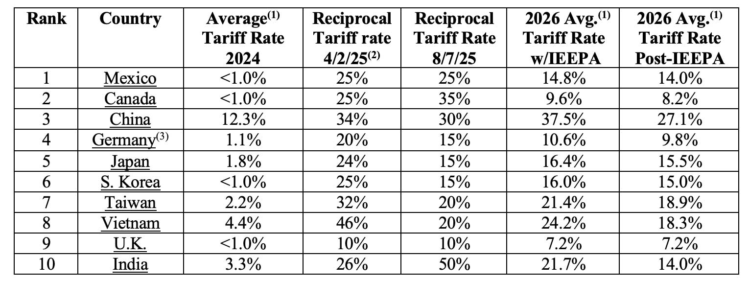
(1) Average tariff rate is trade-weighted; United Nations Trade and Development calculation
(2) Tariff rates for Mexico and Canada were established in March 2025
(3) Tariff rates reflect rate for European Union; Germany is largest EU trading partner
According to the U.S. Treasury, in 2025 tariff revenue comprised of customs duties, taxes, and fees, generated approximately $265 billion in revenue for the federal government, which was approximately 10% of the $2.7 trillion raised through individual income tax revenue. 2025 tariff revenue was approximately 0.7% of the $38.5 trillion federal debt outstanding as of December 31. The regulatory costs of administering the tariff program, including the regulatory costs to the U.S. government of enforcing the tariffs and the regulatory costs to businesses for complying with tariff laws, have not been disclosed nor deducted from tariff revenue numbers. According to the Penn Wharton Budget Model of the University of Pennsylvania, tariff revenue collected under the IEEPA accounted for approximately 50% of total customs duties since the reciprocal tariffs were initiated.
Trade
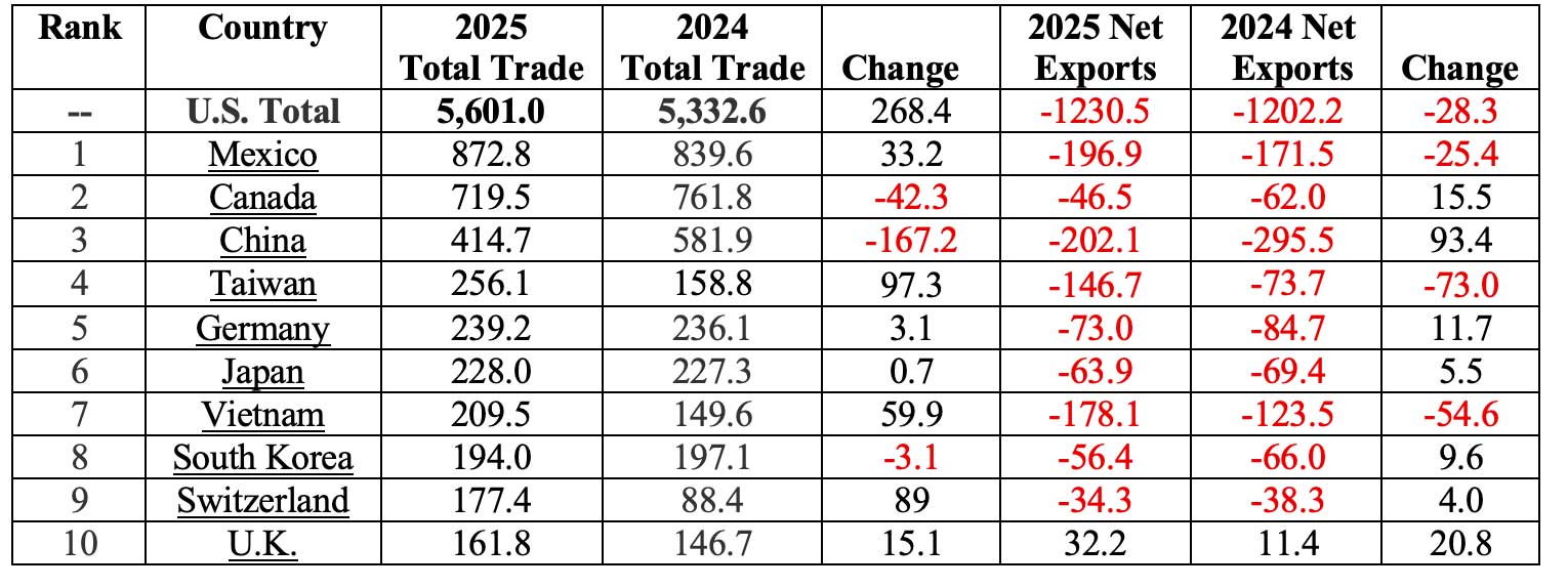
The table below shows the impact of the 2025 tariffs on U.S. trade with its top ten trading partners. The table shows the total trade for 2025 and 2024 with each country, the change in trade, net exports for 2025 and 2024 with each country, and the change in net exports. Net exports are defined as the value of exports minus the value of imports. If net exports are positive, the United States has a trade surplus; if net exports are negative, the United States has a trade deficit. A negative change in net exports means that the trade deficit increased; a positive change means that the trade deficit decreased. In 2025, total trade in goods rose 5.0% to $5.6 trillion. The U.S. trade deficit in goods rose to a record high of $1.23 trillion in 2025, with a 4.3% increase in imports.
In 2025, total trade in goods increased by $268.4 billion while the trade deficit increased by $28.3 billion. The top three trading partners comprised 35.8% of total trade in goods, with Mexico, Canada, and China, accounting for 15.6%, 12.8%, and 7.4% respectively. Trade in goods with the top ten trading partners increased for seven countries, with the largest increases occurring for Taiwan ($97.3 billion) and Vietnam ($59.9 billion). The largest trade decrease was with China, with trade decreasing $167.2 billion. Trade deficits were recorded for nine of the ten top trading partners in 2025, which was identical to 2024. In each year, there was a trade surplus with only the United Kingdom. The largest trade deficit decrease was with China, with a drop of $93.4 billion. Significant trade deficit increases occurred with Taiwan, Vietnam, and Mexico, with increases of $73.0 billion, $54.6 billion, and $25.4 billion, respectively.
2025 Top Ten U.S. Trading Partners in Goods and Changes in Trade
The Labor Market
First, a brief explanation of labor market data and revisions. The Bureau of Labor Statistics (BLS) releases monthly Employment Situation reports, including jobs numbers, on the first Friday of every month. The monthly jobs report reflects preliminary jobs numbers for the previous month based on surveys of employers known as the Current Employment Statistics (CES) survey. The CES survey is a sample of the labor market; it is not a census of the entire labor market. The jobs numbers for a given month are revised based on surveys received after the preliminary numbers have been released. The first revision to jobs numbers occurs one month after the initial release, with a second revision occurring two months after the initial release. In each case, jobs numbers are updated reflecting additional surveys and corrected information received from employers. A monthly household survey (Current Population Survey) is also used by the BLS to derive the unemployment rate.
Once a year, usually in February, the BLS will benchmark the labor market information obtained from employer surveys against the Quarterly Census of Employment and Wages (QCEW), a more complete and accurate measure of labor market data. Additional revisions may occur to prior year jobs numbers. The QCEW is a joint effort between the BLS and state unemployment insurance programs. The QCEW provides a comprehensive tabulation of employment information, and publishes a quarterly count of employment and wages reported by employers covering more than 95 percent of U.S. jobs.
Job Growth
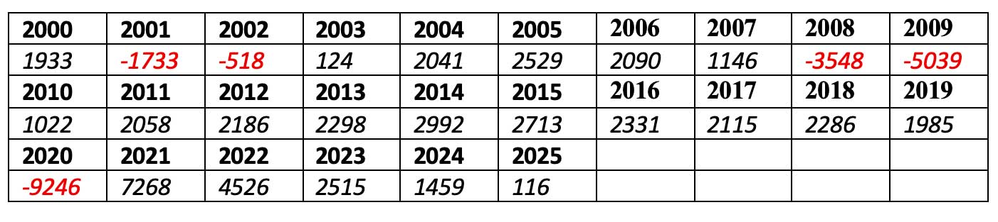
Weak 2025 job growth and a volatile start to 2026 reflected some existing difficulties in the labor market. 2025 was a dismal year for job growth with only 116,000 jobs added, the sixth worst year for job growth this century (with job losses occurring in 2001, 2002, 2008, 2009, and 2020). Five months had job losses. The tables below show annual job growth since 2000 and monthly job growth since January 2025.
Annual Job Growth (in thousands) 2000-2025
Monthly Job Growth (in thousands) January 2025-March 2026
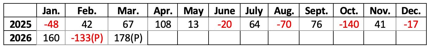
P = Preliminary
In 2026 the jobs market has been volatile. The year began with job gains of 160,000 in January, followed by a preliminary estimate of 133,000 job losses in February. In March, the job market rebounded with a preliminary estimate of 178,000 jobs added.
Total and Industry Employment
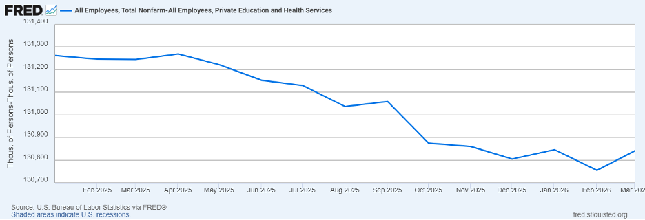
The graph below shows monthly total nonfarm employment minus private education and health services employment over the period January 2025 – March 2026. When private education and health services employment is excluded, total nonfarm employment declined since January 2025. In March 2026, total nonfarm employment excluding private education and health services was 130.842 million, compared to 131.262 million in January 2025, a decrease of 420,000. Over the past twelve months, private education and health services was the number one industry for jobs added with 663,000, a 2.4% gain in industry employment. Leisure and hospitality was second with job gains of 176,000, a 1.0% increase. Government was the leading industry for job losses at 242,000, a 1.0% drop in industry employment. Despite a Trump Administration priority, manufacturing jobs decreased 75,000, or 0.6%.
Total Nonfarm Employees Minus Private Education and Health Services Employees (thousands)
January 2025-March 2026
Job Openings and Private Sector Hires
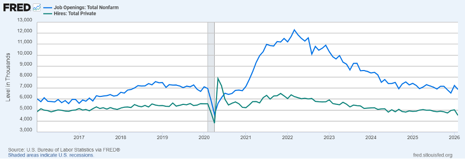
The graph below shows job openings (blue line) and new private sector hires (green line) over a longer-term perspective, the 10-year period from January 2016 through February 2026. The shaded area indicates a period designated recession by the National Bureau of Economic Research. Recent trends in both job openings and new private sector hires generally reflected a softening labor market in 2025. After peaking in early 2022 following the recession, both the number of job openings and the number of private sector hires have fluctuated but generally trended downward. That trend continued in 2025; although job openings increased slightly in early 2026, private sector hires declined.
2025 began with 7.8 million job openings, but the year ended with the fewest job openings since September 2020. The number of openings fell to 6.5 million in December, down from 6.9 million in November. In 2025, the number of private sector job hires peaked in April at 5.3 million before declining to 5.0 million in December. Job openings reached 6.8 million in February 2026, but private sector hires declined to 4.5 million, the lowest level since April 2020.
Job Openings and New Private Sector Hires, thousands
January 2016-February 2026
The Unemployment Rate
The table below shows the unemployment rate since 2022. The unemployment rate is the percentage of unemployed people in the labor force that are willing and available to work and who have actively sought work within the past four weeks. Recently, the benchmark for maximum employment without excessive inflation has been an unemployment rate of 3.5%. Although the unemployment rate has been at relatively low levels since 2022, it generally trended up in 2025. The unemployment rate began the year at 4.0% and ended the year at 4.4%. After fluctuating between 4.0% and 4.5%, the rate appeared to be stabilizing at the end of 2025. Between December 2025 and March 2026, the rate varied between 4.3% and 4.4%. In March 2026, the number of unemployed people was at 7.2 million, similar to the level a year ago.
Annual Job Growth (in thousands) 2000-2025
(Source: Bureau of Labor Statistics)
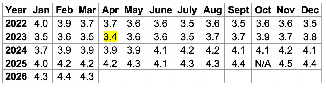
N/A = data is not available due to government shutdown
Monthly low is highlighted in yellow
Permanent Job Losers
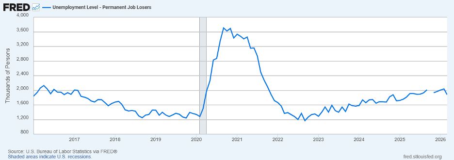
Job losers are defined as individuals who have left their jobs due to various reasons, including layoffs, restructurings, downsizing, and technology. The graph below shows permanent job losers since 2016. Since September 2022, permanent job losers have fluctuated, but the trend is unmistakenly increasing. In 2025 that trend continued, with permanent job losers increasing from 1.72 million in January to 1.97 million in December, the highest level since October 2021. After reaching 2.04 million in February, a slight dip occurred in March 2026 with permanent job losers at 1.88 million. The break in the time series line for October 2025 reflects the absence of data collection due to the government shutdown last year. You will see similar breaks in other charts in this report. The overall growing trend in job cuts in a period of economic growth increases labor market consternation, particularly with the growing presence of AI.
Permanent Job Losers (thousands)
January 2016-March 2026
Duration of Unemployment
The graph below shows the median (blue line) and average (green line) length of unemployment since 2022. Since January 2025 both the median and average length of unemployment have increased, another sign of a challenging labor market. The March 2026 median length of unemployment was the highest level since February 2022, at 11.5 weeks, compared to 10.1 weeks in January 2025. The average length of unemployment rose from 22.0 weeks in January 2026 to 25.3 weeks in March 2026, the highest level in over three years.
Median and Average Duration of Unemployment
January 2022-March 2026
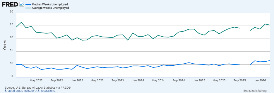
Long-term unemployed, defined as individuals who have been unemployed for 27 weeks or longer and are actively seeking work, increased from 1.449 million in January 2025 to 1.821 million in March 2026.
Oil and Gas Prices
According to the U.S. Energy Information Administration, the United States has had record crude oil production each year since 2023 and led the world in crude oil production since 2018. In 2025, the U.S. produced approximately13.5 million barrels per day of crude oil. However, the U.S. exports and imports crude oil, and overall is a net importer of crude oil, exporting approximately 4 million barrels per day while importing 6.2 million barrels per day. Market economics and differences in domestically produced oil relative to foreign oil are the reasons that the U.S. both exports and imports crude oil.
Crude oil is a raw material that, through processing, is turned into an array of products, including gasoline, diesel, and a wide variety of petroleum products. Oil is a global commodity, but there are generally product differences between domestically produced oil and foreign produced oil. The U.S. imports and exports crude oil because different types of oil are needed to make various products cost effectively. U.S. produced crude oil is generally lighter viscosity than imported foreign produced oil, and some petroleum products may require the heavier foreign oil. The viscosity of oil (light or heavy) and sulfur content (low or high) determine the processes and costs needed to change the oil into a petroleum product. Refineries generally match their processing capabilities with types of crude oils from around the world that enable production of needed domestic products, and products that can be profitably exported. Despite the record U.S. crude oil production, the oil may not match what is needed to make all of the products that Americans use. The top five sources of U.S. crude oil imports by percentage share of U.S. total crude oil imports in 2023 were: Canada (52%), Mexico (11%), Saudi Arabia (5%), Iraq (4%), and Brazil (3%).
Oil is rarely used as a raw commodity for consumption; rather it must be refined into some type of petroleum product. Oil must be produced, refined, and then the manufactured product delivered to where there is consumer demand. Location becomes a key issue for the manufacture of petroleum products, including where the oil is produced, where the refining and manufacturing of products takes place, and where the final product must be shipped. The mix of oil prices, production costs, and transportation costs may make foreign oil cheaper to use in the manufacture of a petroleum product than domestically produced oil when all costs are considered.
Although distinct markets exist for crude oil, oil prices are related due to the potential substitutability of products, and the need for different grades of oil to make needed petroleum products. It’s a global oil market.
There are three prominent benchmarks for oil prices: 1) Brent crude, European oil which is derived from five different oil fields in the North Sea, 2) West Texas Intermediate (WTI) crude, oil extracted from U.S. Wells and sent via pipeline to Cushing, Oklahoma, and 3) Dubai crude, oil from the Middle East. According to Investopedia.com, Brent crude is the most widely used global benchmark for oil pricing, with approximately 80% of global crude contracts tied to the Brent crude oil price. Brent crude is used as the global benchmark due to its quality and relative ease of accessibility. WTI crude is the primary benchmark for the United States, while Dubai crude is the main benchmark for Persian Gulf oil. Both Brent crude and WTI crude are viewed as ideal for the refining of gas and diesel fuel, with Brent crude featuring relative ease of transportation due to its location.
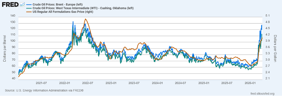
The graph below compares the price for 1) Brent crude (blue line, left-axis), 2) WTI crude (green line, left-axis), and 3) U.S. regular gas (brown line, right axis), over the period from January 2021 through early April 2026. Although differences exist between oil markets due to demand and supply differences that exist within the specific markets, the overall ups and downs of Brent crude (Europe) oil prices and WTI crude (U.S.) oil prices are strongly related, indicating a global energy market. Similarly, although differences exist in the factors that affect each market, the overall trend in changes in gas prices strongly reflects the overall trend in changes in oil prices. There is a strong relationship in the overall trend, with increasing gas prices generally reflecting increasing oil prices and decreasing gas prices reflecting decreasing oil prices.
Oil prices spiked in early 2022 with Brent crude at approximately $130 per barrel due to the Russian invasion of Ukraine. Although a general downward trend began in late 2022, oil prices rebounded in 2023 due to Middle East turbulence and OPEC production cuts before declining in 2024 and 2025. Brent crude fell to approximately $75 per barrel at the end of 2024 and $62 per barrel to close out 2025. That trend reversed in 2026 due to the U.S. war in Iran. Since the start of the year, the price of Brent crude approximately doubled to over $125/barrel in early April while gas prices soared to over $4 per gallon.
Brent Crude (Europe) Oil Price vs. WTI Crude Oil Price (U.S.) vs. U.S. Gas Prices
January 2021-April 6, 2026
Inflation
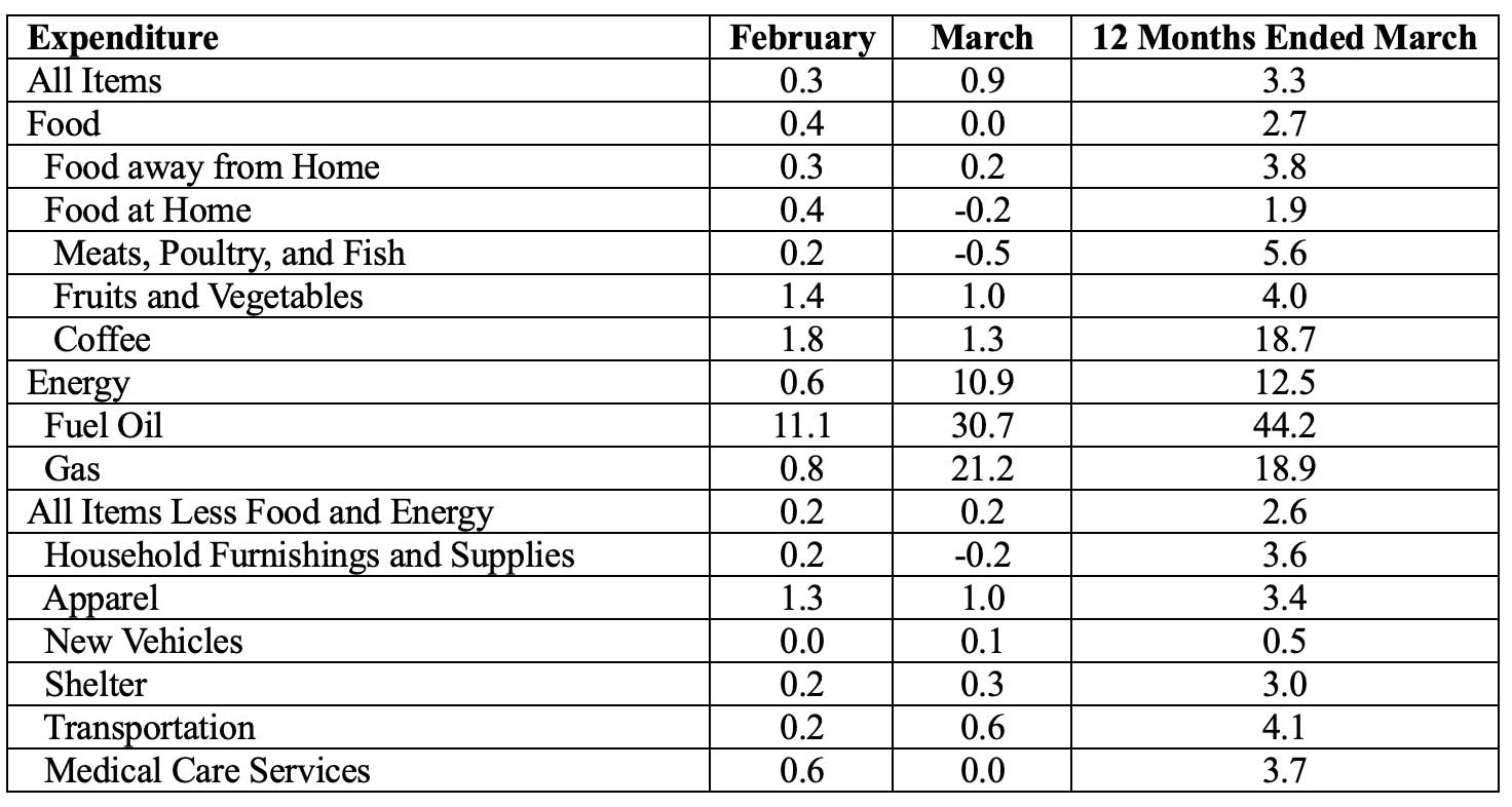
Inflation was 3.3% for the 12 months ended March 2026, but the spike in March energy prices caused by the Iran war led to a 0.9% surge in inflation just for the month of March. Overall energy prices spiked in March, rising 10.9% led by sharp increases in fuel oil (30.7%) and gas (21.2%). The one-month rise in gas was the largest since 1967 when monthly price changes were first published. Rising oil and energy prices can have a rippling effect through the U.S. economy, increasing not only gas prices, but also manufacturing costs, agricultural costs, shipping costs and travel prices. The rippling effect will take some time to filter through the economy, but rising price fuel and gas prices does not bode well for future product and service prices.
For the 12-months ended March, overall food prices rose 2.7% with consumers particularly stressed by significant increases in several food products. Meat, poultry, and fish prices were up 5.6%, fruits and vegetables increased 4.0%, and coffee skyrocketed 18.1%. Transportation prices bumped up 0.6% in March alone, a refection of rising fuel costs. For the 12-months ended March, transportation prices rose 4.1%, with price increases of greater than 3% for household furnishings and supplies (3.6%), medical care services (3.7%), and apparel (3.4%). Shelter increased 3.0%. Listed below is the one-month price change for February and March for selected expenditure categories, as well as the price change for the 12-months ended March 2026.
CPI by Expenditure Category, Feb. and March 2026 One-Month (seasonally adj.) Changes
12-month Change for Period Ending March 2026
The graph below shows the annualized U.S. inflation rate from January 2024 through March 2026 as measured by the twelve-month change in the Consumer Price Index (CPI) for all items (blue line) and the Consumer Price Index, less Food and Energy (green line). Stripping out the relatively volatile categories of food and energy from the Consumer Price Index provides a measure of core inflation.
Percent Change in CPI and CPI Less Food and Energy from One Year Ago
January 2024-March 2026
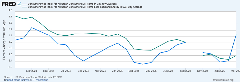
From January 2024 through September 2024 overall inflation generally declined, with the CPI declining from 3.5% in March 2024 to 2.4% in September 2024, before gradually ticking up to 3.0% in January 2025. Inflation trended downward once again as 2025 began, decreasing to 2.3% in April, but steadily increased to 3.0% in September before dropping down to 2.4% in January 2026. The spike in energy prices led to a surge in inflation in March to 3.3%, the highest level since April 2024. Core inflation, measured by stripping out the relatively volatile food and energy categories from the CPI all items index, rose from 2.5% in February 2026 to 2.6% in March, after generally declining from a 3.1% rate in August 2025.
After inflation fluctuating around 2% for most of the last decade, the Federal Reserve’s inflationary goal of 2% has been elusive this decade. While it may take some time for the impact of changing energy prices and tariffs to filter through the economy, certainly the March spike in energy prices and continuing tariffs won’t make the Federal Reserve’s goal easier to achieve. The Yale Budget Lab estimated that the tariff policies in effect as of April 8 will increase prices by 0.7% if section 122 tariffs expire in July or 1.1% if section 122 tariffs are extended, assuming the tariff costs are passed through to consumers. This results in an approximate loss of $940 (section 122 tariffs expire) or $1,500 (section 122 tariffs extended) for the average household.
Economic Growth
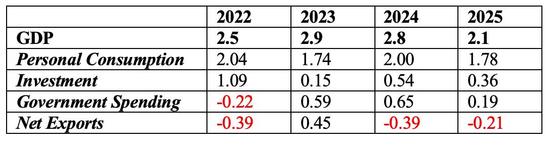
Economic growth continued but slowed in 2025. The table below shows how changes in the four components of Gross Domestic Product (GDP) contributed to the change in U.S. economic growth since 2022. Economic growth is measured by changes in GDP, which is the value of goods and services produced in a given time period. After growth of 2.5 percent, 2.9 percent, and 2.8 percent in 2022, 2023, and 2024, respectively, economic growth slowed to 2.1 percent in 2025.
As indicated in the chart below, personal consumption has been the key and consistent driver of economic growth. Personal consumption accounts for approximately two-thirds of Gross Domestic Product, and contributed significantly more to GDP growth than investment spending (including business investment in equipment and inventories), government spending, or net exports in every year.
Contributions to Percent Change in Real Gross Domestic Product–Annualized Rate
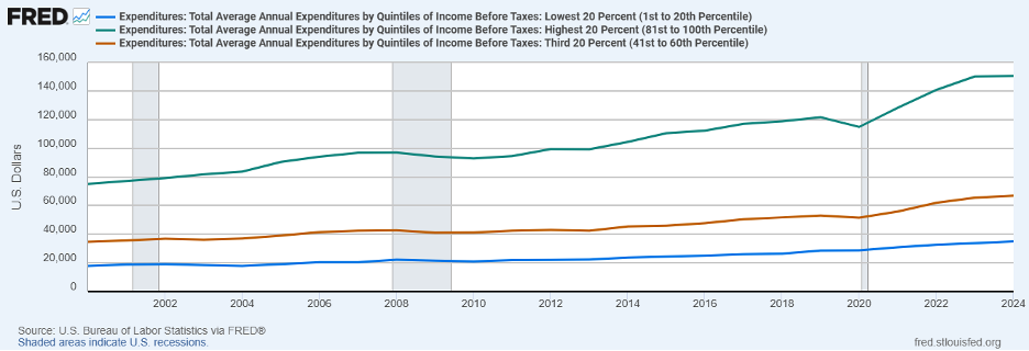
Higher income households have driven the growth in consumer spending, particularly since 2020. The graph below compares total average annual expenditures of higher income households (green line, 81st to 100th income percentile), middle income households (brown line, 41st to 60th income percentile), and lower income households (blue line, 1st to 20th income percentile) over the period 2000-2024. (2025 data is not available due to the government shutdown).
Since 2020, total average expenditures for higher income households rose from $114,839 to $150,342, an increase of $35,503 or 30.9%. Total average expenditures for middle income households rose from $51,554 to $66,900, a gain of $15,346 or 29.7%. Total average expenditures for lower income households increased from $28,732 to $35,046, an increase of $6,314 or 21.9%. Expenditures were aided by a strong stock market and differential wage growth, which contributed to an evolving K-shaped economy. According to the Congressional Research Service, over the 10-year period 2014-2024, annual real wages grew from approximately $26,000 to $32,000 for workers at the 10th percentile of the wage distribution, from $52,000 to $58,000 for workers at the median, and from $122,000 to $140,000 for workers at the 90th percentile.
Total Average Expenditures by Quartiles of Household Income
2000-2024
The Financial Markets
The Stock Market
The U.S. stock market reflects expectations for future economic performance and corporate profitability. In 2025, the S&P 500, a broad benchmark index for U.S. large company (large-cap) stocks, rose to record highs. However, in a major shift for stock market performance, the U.S. stock market lagged behind most major foreign stock markets. That trend continued in the first quarter of 2026.
The table below compares major stock index returns for selected countries for 2024, 2025, the 5-years (annualized) ending December 31, 2025, and the first quarter of 2026. The selected indexes are broad measures of stock market performance in their respective countries. The U.S. S&P 500 is a leading benchmark index for U.S. large company (large-cap) stocks, with a long-run historical annual average return of approximately 10 percent. The U.S. stock market soared in 2024, with returns more than twice the historical average. In 2024, the U.S. stock market was the leader of the pack, outperforming every other index listed below with the S&P 500 returning 23.31 percent.
That trend reversed in 2025. Although the S&P 500 reached record highs, the U.S. stock market lagged behind several foreign stock markets. In 2025 the U.S. S&P 500 returned 16.39 percent, significantly higher than the historical average, but lower than the returns of several foreign stock markets. Despite the U.S. imposed tariffs in 2025, the stock market performance of Mexico, Canada, the United Kingdom, Germany, Japan, and China exceeded the performance of the S&P 500. The stock markets of America’s top three trading partners – Mexico, Canada, and China, all outperformed the S&P 500 despite significant U.S. tariffs. Canada and Mexico vastly outperformed, with stock market returns of 28.93 percent and 25.17 percent, respectively, compared to the 16.39 percent for the U.S. The 2025 Canadian stock market performance propelled it to the top spot for 5-year returns, with annualized returns of 13.27 percent. The U.S. ranked third in 5-year returns, with annualized returns of 12.75 percent.
The Iran war and skyrocketing oil prices weighed heavily on global stock markets and economic uncertainty in the first quarter of 2026. The S&P 500 declined 4.63 percent, with only Germany performing worse with a drop of 7.39 percent. Four of the nine countries listed below had stock market increases, including Canada, Mexico, the United Kingdom, and Japan. The Mexican stock market was by far the top performer with an increase of 8.11 percent, with Canada a distant second posting a gain of 3.19 percent.
Global Stock Market Performance of Selected Indexes
2024, 2025, Five-Year Returns (annualized) as of December 31, 2025, and First Quarter 2026

Artificial intelligence was a key driver of U.S. stock market gains prior to 2026. In the first quarter of 2026, AI propelled stock market losses. The Morningstar Global Artificial Intelligence Select Index includes stocks of 48 major companies with exposure to generative AI, AI data & infrastructure, AI software, and AI services. The index rose 75.27 percent and 34.78 percent in 2023 and 2024, respectively, with another 30.84 percent increase in 2025. The Nasdaq Composite Index includes over 2,500 stocks and is a key indicator of tech sector stock market performance. Driven by AI, the Nasdaq was up 20.36 percent in 2025, following increases of 43.42 percent and 28.64 percent in 2023 and 2024, respectively. Economic uncertainty in the first quarter of 2026 cooled AI optimism, and the Morningstar Global Artificial Intelligence Select Index declined 4.81 percent while the Nasdaq dropped 7.11 percent. The S&P 500 was also impacted, as it has significant exposure to AI. Five tech-heavy stocks comprise over 25 percent of S&P 500 market capitalization (total stock value): 1) Apple, 2) Nvidia, 3) Microsoft, 4) Alphabet, and 5) Amazon.
Interest Rates
The Federal Reserve is the key driver of short-term interest rates in the United States economy through its monetary policy, which is implemented primarily through targeting the federal (fed) funds rate. The fed funds rate is the overnight borrowing rate between banks, a very short-term interest rate that when changed, typically has a rippling effect throughout financial markets. The Federal Reserve influences the fed funds rate primarily by controlling the money supply in the United States. The amount of money circulating in the economy has an impact on interest rates and credit conditions – more money, lower interest rates; less money, higher interest rates. Changes in the fed funds rate generally affect savings and borrowing rates, although the Federal Reserve’s monetary policy is not the only factor that influences savings and borrowing rates.
The Federal Reserve, since 1977, has had a dual mandate of achieving maximum employment and price stability. To achieve these goals, the Federal Reserve acts in a nonpartisan, independent manner to balance economic growth (which affects employment) with inflation. Lower interest rates can increase consumer and business spending which fuels economic growth and boosts employment. However, too much economic growth, or economic growth when the economy is near full employment, can increase inflation. Higher interest rates can lower economic growth by reducing interest rate sensitive consumer and business spending, which generally lowers the demand for products and services and consequently inflation. To achieve price stability, the Federal Reserve has stated that an inflation rate of 2% over the longer run, as measured by the annual change in the price index for personal consumption expenditures, is most consistent with the Fed’s price mandate.
The Federal Reserve cut interest rates three times in 2025, beginning in September. 2025 was a challenging year for the Federal Reserve, as the uncertainties of the impact of tariffs on inflation contrasted with a softening labor market, created a dichotomy for the direction of Federal Reserve policy. In September, in response to the softening labor market, the Federal Reserve implemented its first rate cut of the year, lowering the fed funds rate by 25 basis points to a target range of 4.00-4.25. Two more 25-basis point cuts occurred in October and December, lowering the fed funds target range to 3.50-3.75. No rate cuts occurred in the first quarter of 2026.
On May 15, 2026, the term of the current Chairman of the Federal Reserve, Jerome Powell, is scheduled to end. President Trump has clearly indicated that he favors more interest rate cuts from the next Fed chair. In 2026 the Federal Reserve has been reluctant to cut interest rates further, as the combination of tariffs and spike in energy costs due to the Iran war created increased inflationary concerns. Inflation remains above the Fed’s target 2% level. The process for selecting the next Chair, who serves a four-year term, involves being nominated by the President and then confirmed by the Senate. Exactly how that process will play out remains to be seen. The financial markets have generally viewed the ability of the Federal Reserve to operate independently, without interference from Congress or the President, as critically important to the long-term growth of the United States economy and financial market performance. The degree of future Federal Reserve independence also remains to be seen.
U.S. Debt and Deficits
Except for a brief period between 1998 and 2001 when the U.S. was enjoying excellent economic growth and the tech boom in its internet infancy, the United States has had budget deficits since 1980. To finance a budget deficit, the government borrows money from the public through the issuance of U.S. government debt called U.S. Treasury securities. The Total Public (Federal) Debt Outstanding represents the total (principal) amount of Treasury securities outstanding issued by the federal government. Generally, the public (federal) debt outstanding reflects the accumulation of budget deficits, with subsequent budget deficits increasing the total public (federal) debt outstanding. The graph below shows the relationship between federal budget deficits and the total public (federal) debt. The blue line (left axis) indicates the total federal debt outstanding; the green line (right axis) shows the budget deficits or surpluses that have occurred since 1980. Growing federal debt is becoming an increasing problem for the United States and threatens future program funding, including mandatory programs (including Social Security, Medicare, and Medicaid), and discretionary programs (defense and nondefense programs).
Federal Budget Surplus or Deficit; Total Public Debt 1980-2025
(millions of dollars)
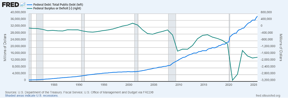
Major events that played a role in significantly increasing the budget deficit and federal debt include: 1) tax cuts (2003 and 2018), 2) the financial crisis of 2008, and 3) the COVID crisis of 2020. Despite an expanding economy with an unemployment rate hovering around only 3.5%, in 2019 the budget deficit doubled from its 2015 level to over $983 billion. Between 2019 and 2025, the deficit nearly doubled again, ending fiscal year 2025 at $1.775 trillion. Between 1980 and 2010, federal debt rose from approximately $1 trillion to $13 trillion. Since 2010, the debt has approximately tripled to $38.5 trillion in 2025, a record high. Between 2025-2034, the One Big Beautiful Bill is estimated by the Congressional Budget Office to increase the deficit by over $4 trillion.
The growing federal debt will add to forthcoming political and budget battles over the mix of fiscal spending, including Social Security. Social Security and Medicare are funded by federal taxes paid by employers and employees. Payroll taxes provide over 90% of Social Security program income. (Additional program income includes taxation of Social Security benefits and interest on trust fund assets.) Employees and their employers each pay 6.2% of earnings for Social Security taxes; an additional 1.45% of earnings are paid for Medicare taxes. In sum, a total of 15.30% of an employee’s earnings are subject to Social Security and Medicare taxes, with employee and employer each paying 7.65% of an employee’s earnings. There is a salary limit for Social Security taxes. The salary limit is $184,500 in 2026, with the salary limit typically adjusted each year by the approximate level of inflation. (There is no salary limit for Medicare taxes.) Earnings exceeding the salary limit are not subject to Social Security taxes. The formula to determine a worker’s Social Security benefit is a function of the payroll taxes paid to Social Security. The primary purpose of Social Security retirement benefits is to provide a base level of economic security, not to provide a high rate of return on the payroll taxes paid in by workers.
Current payments into Social Security are being dispersed to those receiving benefits now – excess payments, if any, remain in Social Security trust funds. In 2021, Social Security’s total cost exceeded its total income for the first time since 1982. Disbursements are expected to continue to exceed program income for the foreseeable future, with money drawn from the trust funds to pay the difference. Current payments into Social Security being dispersed to current beneficiaries set the stage for financial difficulties when the demographics of the U.S. shifted to an aging population. According to the Social Security Trustees, the trust fund for Social Security retirement income will be depleted in 2032. The One Big Beautiful Bill accelerated the trust fund depletion by reducing taxes on Social Security benefits, which were used to help fund the program. Under current law, when the trust fund is depleted, payments to beneficiaries will be limited to program income. In 2033, that is expected to result in an approximate 23% cut in Social Security to recipients – unless current laws change. The average monthly Social Security benefit for retired workers was $1,976 in 2025. The Medicare trust fund is also under financial duress, and expected to be insolvent by 2033.
The Congressional Budget Office (CBO) is a nonpartisan federal agency that provides independent economic and budget analysis to the United States Congress. The CBO projects that from 2026 to 2036, based on current laws, large and growing deficits will cause federal debt to increase substantially. The deficit is expected to grow from $1.8 trillion in fiscal year 2025 to $3.1 trillion in 2036 with federal debt increasing from $38.5 trillion at the end of 2025 to $56 trillion in 2036. The CBO states that “budget projections continue to indicate that the fiscal trajectory is not sustainable.” The aging of the population increases expected Social Security payments, from $1.7 trillion in 2026 to $2.7 trillion in 2036, with Medicare approximately doubling from $1.0 trillion in 2026 to $2.0 trillion in 2036. The expected depletion of the Social Security retirement trust fund in 2032, which requires program cuts to beneficiaries unless current laws change, is rapidly approaching. The growth in federal debt and pending exhaustion of Social Security and Medicare trust funds is on a collision course. The outcome should be interesting.
For further information:
- From the Budget Lab at Yale University: Trade and Tariffs
- From the Penn Wharton Budget Model: Supreme Court Ruling and IEEPA Revenue
- From the U.N. Trade and Development: Tariff dashboard – tracking the evolution of US tariffs | UN Trade and Development (UNCTAD)
- From the U.S. Census Bureau and Bureau of Economic Analysis: U.S. International Trade
- From the U.S. Census Bureau:
- Info from the Bureau of Labor Statistics:
- From the Congressional Research Service: Recent Wages Trends and Issues | Congress.gov | Library of Congress
- Federal Reserve Economic Data (FRED) for West Texas Intermediate oil prices: West Texas Intermediate Oil Prices
- From the U.S. Energy Information Administration:
- From Investopedia.com: Benchmark Oils: Brent Crude, WTI, and Dubai
- GDP Growth (and other national data) from the Bureau of Economic Analysis: GDP Growth
- From Morningstar:
- CME FedWatch Tool: CME Fed Funds Futures
- From the Federal Reserve: Open Market Operations and the Fed Funds Rate
- The Federal Budget from the Congressional Budget Office (CBO): The Budget and Economic Outlook: 2026 to 2036 | Congressional Budget Office
- A summary of the financial status of Social Security from the Trustees: https://www.ssa.gov/OACT/TRSUM/index.html

Kevin Bahr is a professor emeritus of finance and chief analyst of the Center for Business and Economic Insight in the Sentry School of Business and Economics at the University of Wisconsin-Stevens Point.